CMIP6 Emulation
[1]:
import numpy as np
import pandas as pd
import matplotlib.pyplot as plt
from esem import gp_model
from esem.utils import validation_plot
%matplotlib inline
[2]:
df = pd.read_csv('CMIP6_scenarios.csv', index_col=0).dropna()
[3]:
# These are the models included
df.model.unique()
[3]:
array(['CanESM5', 'ACCESS-ESM1-5', 'ACCESS-CM2', 'MPI-ESM1-2-HR',
       'MIROC-ES2L', 'HadGEM3-GC31-LL', 'UKESM1-0-LL', 'MPI-ESM1-2-LR',
       'CESM2', 'CESM2-WACCM', 'NorESM2-LM'], dtype=object)
[4]:
# And these scenarios
df.scenario.unique()
[4]:
array(['ssp126', 'ssp119', 'ssp245', 'ssp370', 'ssp585', 'ssp434'],
      dtype=object)
[5]:
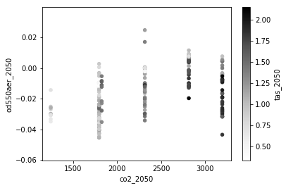
ax = df.plot.scatter(x='co2_2050', y='od550aer_2050', c='tas_2050')
[6]:
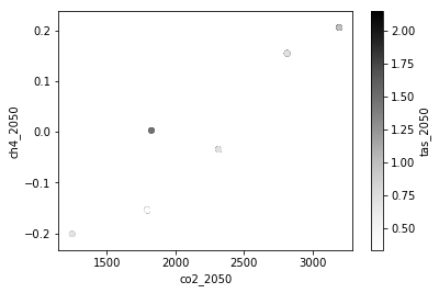
ax = df.plot.scatter(x='co2_2050', y='ch4_2050', c='tas_2050')
[7]:
# Collapse ensemble members
df = df.groupby(['model', 'scenario']).mean()
df
[7]:
| tas_2050 | od550aer_2050 | tas_2100 | od550aer_2100 | co2_2050 | co2_2100 | so2_2050 | so2_2100 | ch4_2050 | ch4_2100 | ||
|---|---|---|---|---|---|---|---|---|---|---|---|
| model | scenario | ||||||||||
| ACCESS-CM2 | ssp126 | 1.000582 | -0.025191 | 1.407198 | -0.038552 | 1795.710867 | 1848.864201 | -0.064020 | -0.082066 | -0.153999 | -0.241390 |
| ssp245 | 1.187015 | -0.012222 | 2.489487 | -0.027589 | 2314.385253 | 3932.717046 | -0.035997 | -0.059775 | -0.034673 | -0.092845 | |
| ssp370 | 1.103402 | 0.006077 | 3.791109 | 0.001188 | 2813.146604 | 6912.965613 | 0.004142 | -0.020179 | 0.154481 | 0.368859 | |
| ssp585 | 1.478602 | -0.008842 | 5.016310 | -0.016805 | 3192.373467 | 10283.292188 | -0.028185 | -0.059536 | 0.205365 | 0.104140 | |
| ACCESS-ESM1-5 | ssp126 | 0.819904 | -0.013947 | 0.967981 | -0.015895 | 1795.710867 | 1848.864201 | -0.064020 | -0.082066 | -0.153999 | -0.241390 |
| ssp245 | 1.078853 | -0.004727 | 2.052867 | -0.009796 | 2314.385253 | 3932.717046 | -0.035997 | -0.059775 | -0.034673 | -0.092845 | |
| ssp370 | 1.047218 | 0.003862 | 3.422980 | 0.000495 | 2813.146604 | 6912.965613 | 0.004142 | -0.020179 | 0.154481 | 0.368859 | |
| ssp585 | 1.412020 | -0.002210 | 4.096812 | -0.001356 | 3192.373467 | 10283.292188 | -0.028185 | -0.059536 | 0.205365 | 0.104140 | |
| CESM2 | ssp126 | 0.974787 | -0.003323 | 1.134402 | -0.010735 | 1795.710867 | 1848.864201 | -0.064020 | -0.082066 | -0.153999 | -0.241390 |
| ssp245 | 1.119462 | 0.000371 | 2.303586 | 0.000121 | 2314.385253 | 3932.717046 | -0.035997 | -0.059775 | -0.034673 | -0.092845 | |
| ssp370 | 1.154434 | 0.007554 | 3.501974 | 0.016237 | 2813.146604 | 6912.965613 | 0.004142 | -0.020179 | 0.154481 | 0.368859 | |
| ssp585 | 1.453782 | 0.002178 | 4.980513 | 0.016340 | 3192.373467 | 10283.292188 | -0.028185 | -0.059536 | 0.205365 | 0.104140 | |
| CESM2-WACCM | ssp126 | 0.770853 | 0.000561 | 1.053462 | -0.006278 | 1795.710867 | 1848.864201 | -0.064020 | -0.082066 | -0.153999 | -0.241390 |
| ssp245 | 1.118329 | 0.000520 | 2.252389 | 0.006330 | 2314.385253 | 3932.717046 | -0.035997 | -0.059775 | -0.034673 | -0.092845 | |
| ssp370 | 1.022903 | 0.011563 | 3.526784 | 0.035894 | 2813.146604 | 6912.965613 | 0.004142 | -0.020179 | 0.154481 | 0.368859 | |
| ssp585 | 1.311378 | 0.005453 | 5.010599 | 0.038768 | 3192.373467 | 10283.292188 | -0.028185 | -0.059536 | 0.205365 | 0.104140 | |
| CanESM5 | ssp119 | 0.641977 | -0.030857 | 0.333723 | -0.036624 | 1247.788346 | 905.867767 | -0.069425 | -0.080790 | -0.201275 | -0.257405 |
| ssp126 | 0.989167 | -0.029769 | 0.953098 | -0.041451 | 1795.710867 | 1848.864201 | -0.064020 | -0.082066 | -0.153999 | -0.241390 | |
| ssp245 | 1.318495 | -0.016138 | 2.454336 | -0.033573 | 2314.385253 | 3932.717046 | -0.035997 | -0.059775 | -0.034673 | -0.092845 | |
| ssp370 | 1.724648 | -0.004288 | 4.744037 | -0.021374 | 2813.146604 | 6912.965613 | 0.004142 | -0.020179 | 0.154481 | 0.368859 | |
| ssp434 | 1.304015 | -0.023741 | 1.863815 | -0.040477 | 1825.355018 | 1612.733274 | -0.055372 | -0.077382 | 0.002907 | -0.032744 | |
| ssp585 | 1.877571 | -0.025367 | 5.984793 | -0.040852 | 3192.373467 | 10283.292188 | -0.028185 | -0.059536 | 0.205365 | 0.104140 | |
| HadGEM3-GC31-LL | ssp126 | 0.768553 | -0.026508 | 1.314000 | -0.037692 | 1795.710867 | 1848.864201 | -0.064020 | -0.082066 | -0.153999 | -0.241390 |
| ssp245 | 1.262740 | -0.014397 | 2.651430 | -0.024341 | 2314.385253 | 3932.717046 | -0.035997 | -0.059775 | -0.034673 | -0.092845 | |
| ssp585 | 1.606117 | -0.007902 | 5.547793 | -0.015396 | 3192.373467 | 10283.292188 | -0.028185 | -0.059536 | 0.205365 | 0.104140 | |
| MIROC-ES2L | ssp119 | 0.703733 | -0.014334 | 0.557255 | -0.020002 | 1247.788346 | 905.867767 | -0.069425 | -0.080790 | -0.201275 | -0.257405 |
| ssp126 | 0.785037 | -0.017767 | 0.572429 | -0.028761 | 1795.710867 | 1848.864201 | -0.064020 | -0.082066 | -0.153999 | -0.241390 | |
| ssp245 | 0.789146 | -0.010066 | 1.589075 | -0.019236 | 2314.385253 | 3932.717046 | -0.035997 | -0.059775 | -0.034673 | -0.092845 | |
| ssp370 | 1.131194 | 0.001314 | 2.623115 | 0.006749 | 2813.146604 | 6912.965613 | 0.004142 | -0.020179 | 0.154481 | 0.368859 | |
| ssp585 | 1.117971 | -0.003265 | 3.748485 | -0.003236 | 3192.373467 | 10283.292188 | -0.028185 | -0.059536 | 0.205365 | 0.104140 | |
| MPI-ESM1-2-HR | ssp126 | 0.370221 | -0.009666 | 0.351424 | -0.014088 | 1795.710867 | 1848.864201 | -0.064020 | -0.082066 | -0.153999 | -0.241390 |
| ssp245 | 0.735819 | -0.001871 | 1.352010 | -0.008150 | 2314.385253 | 3932.717046 | -0.035997 | -0.059775 | -0.034673 | -0.092845 | |
| ssp370 | 0.819827 | 0.008950 | 2.616101 | 0.003430 | 2813.146604 | 6912.965613 | 0.004142 | -0.020179 | 0.154481 | 0.368859 | |
| ssp585 | 0.946618 | 0.004603 | 3.153594 | -0.004407 | 3192.373467 | 10283.292188 | -0.028185 | -0.059536 | 0.205365 | 0.104140 | |
| MPI-ESM1-2-LR | ssp126 | 0.518146 | -0.009654 | 0.358184 | -0.014067 | 1795.710867 | 1848.864201 | -0.064020 | -0.082066 | -0.153999 | -0.241390 |
| ssp370 | 0.877299 | 0.008940 | 2.610222 | 0.003437 | 2813.146604 | 6912.965613 | 0.004142 | -0.020179 | 0.154481 | 0.368859 | |
| ssp585 | 1.029724 | 0.004613 | 3.278956 | -0.004377 | 3192.373467 | 10283.292188 | -0.028185 | -0.059536 | 0.205365 | 0.104140 | |
| NorESM2-LM | ssp126 | 0.331449 | -0.011588 | 0.376486 | -0.017219 | 1795.710867 | 1848.864201 | -0.064020 | -0.082066 | -0.153999 | -0.241390 |
| ssp245 | 0.533042 | -0.001380 | 1.295670 | -0.005419 | 2314.385253 | 3932.717046 | -0.035997 | -0.059775 | -0.034673 | -0.092845 | |
| ssp370 | 0.704050 | 0.007691 | 2.552758 | 0.022834 | 2813.146604 | 6912.965613 | 0.004142 | -0.020179 | 0.154481 | 0.368859 | |
| ssp585 | 0.983765 | 0.007667 | 2.957163 | 0.009652 | 3192.373467 | 10283.292188 | -0.028185 | -0.059536 | 0.205365 | 0.104140 | |
| UKESM1-0-LL | ssp119 | 0.918189 | -0.027682 | 0.970074 | -0.035182 | 1247.788346 | 905.867767 | -0.069425 | -0.080790 | -0.201275 | -0.257405 |
| ssp126 | 1.284645 | -0.024166 | 1.563342 | -0.036149 | 1795.710867 | 1848.864201 | -0.064020 | -0.082066 | -0.153999 | -0.241390 | |
| ssp245 | 1.604553 | -0.010934 | 3.040434 | -0.022142 | 2314.385253 | 3932.717046 | -0.035997 | -0.059775 | -0.034673 | -0.092845 | |
| ssp370 | 1.749074 | 0.004618 | 5.046036 | 0.007180 | 2813.146604 | 6912.965613 | 0.004142 | -0.020179 | 0.154481 | 0.368859 | |
| ssp434 | 1.511831 | -0.009184 | 2.371976 | -0.027848 | 1825.355018 | 1612.733274 | -0.055372 | -0.077382 | 0.002907 | -0.032744 | |
| ssp585 | 2.028151 | -0.007564 | 6.038747 | -0.006429 | 3192.373467 | 10283.292188 | -0.028185 | -0.059536 | 0.205365 | 0.104140 |
[8]:
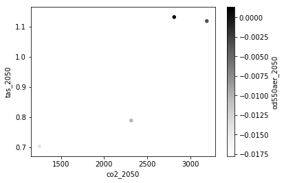
ax = df.query("model == 'MIROC-ES2L'").plot.scatter(x='co2_2050', y='tas_2050', c='od550aer_2050')
[9]:
from utils import normalize
# Merge the year columns in to a long df
df=pd.wide_to_long(df.reset_index(), ["tas", "od550aer", "co2", "ch4", "so2"], i=['model', 'scenario'], j="year", suffix='_(\d+)')
# Choose only the 2050 data since the aerosol signal is pretty non-existent by 2100
df = df[df.index.isin(["_2050"], level=2)]
[10]:
df.describe()
[10]:
| tas | od550aer | co2 | ch4 | so2 | |
|---|---|---|---|---|---|
| count | 47.000000 | 47.000000 | 47.000000 | 47.000000 | 47.000000 |
| mean | 1.085538 | -0.006851 | 2415.708964 | 0.024789 | -0.035145 |
| std | 0.381735 | 0.011775 | 613.880074 | 0.152382 | 0.025320 |
| min | 0.331449 | -0.030857 | 1247.788346 | -0.201275 | -0.069425 |
| 25% | 0.804487 | -0.014140 | 1795.710867 | -0.153999 | -0.064020 |
| 50% | 1.047218 | -0.004727 | 2314.385253 | -0.034673 | -0.035997 |
| 75% | 1.307697 | 0.003020 | 2813.146604 | 0.154481 | -0.028185 |
| max | 2.028151 | 0.011563 | 3192.373467 | 0.205365 | 0.004142 |
[11]:
# Do a 20/80 split of the data for test and training
msk = np.random.rand(len(df)) < 0.8
train, test = df[msk], df[~msk]
Try a few different models
[12]:
from esem.utils import leave_one_out, prediction_within_ci
from scipy import stats

# Try just modelling the temperature based on cumulative CO2
res = leave_one_out(df[['co2']], df[['tas']].values, model='GaussianProcess', kernel=['Linear'])

r2_values = stats.linregress(*np.squeeze(np.asarray(res, dtype=float)).T[0:2])[2]**2
print("R^2: {:.2f}".format(r2_values))
validation_plot(*np.squeeze(np.asarray(res, dtype=float)).T)
R^2: 0.25
Proportion of 'Bad' estimates : 2.13%
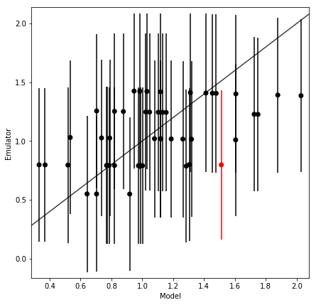
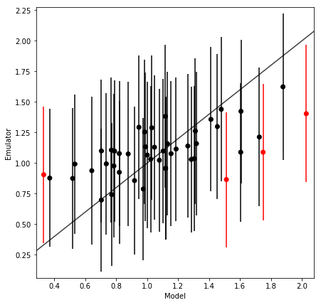
[13]:
# This model still doesn't do brilliantly, but it's better than just CO2
res = leave_one_out(df[['co2', 'od550aer']], df[['tas']].values, model='GaussianProcess', kernel=['Linear'])

r2_values = stats.linregress(*np.squeeze(np.asarray(res, dtype=float)).T[0:2])[2]**2
print("R^2: {:.2f}".format(r2_values))
validation_plot(*np.squeeze(np.asarray(res, dtype=float)).T)
R^2: 0.40
Proportion of 'Bad' estimates : 8.51%
[14]:
# Adding Methane doesn't seem to improve the picture
res = leave_one_out(df[['co2', 'od550aer', 'ch4']], df[['tas']].values, model='GaussianProcess', kernel=['Linear', 'Bias'])

r2_values = stats.linregress(*np.squeeze(np.asarray(res, dtype=float)).T[0:2])[2]**2
print("R^2: {:.2f}".format(r2_values))
validation_plot(*np.squeeze(np.asarray(res, dtype=float)).T)
R^2: 0.40
Proportion of 'Bad' estimates : 8.51%

Plot the best
[15]:
m = gp_model(df[['co2', 'od550aer']], df[['tas']].values, kernel=['Linear'])
m.train()
[16]:
# Sample a large AOD/CO2 space using the emulator
xx, yy = np.meshgrid(np.linspace(0, 4000, 25), np.linspace(-.05, 0.05, 20))
X_new = np.stack([xx.flat, yy.flat], axis=1)
Y_new, Y_new_sigma = m.predict(X_new)
[17]:
# Calculate the scnario mean values for comparison
scn_mean = train.groupby(['scenario']).mean()
[18]:
import matplotlib
scale = 1.5
matplotlib.rcParams['font.size'] = 12 * scale
matplotlib.rcParams['lines.linewidth'] = 1.5 * scale
matplotlib.rcParams['lines.markersize'] = 6 * scale
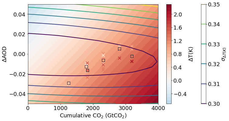
plt.figure(figsize=(12, 6))
norm = matplotlib.colors.Normalize(vmin=-2.5,vmax=2.5)
p = plt.contourf(xx, yy, Y_new.reshape(xx.shape), norm=norm, levels=30, cmap='RdBu_r')
plt.scatter(train.co2, train.od550aer, c=train.tas, norm=norm, edgecolors='k', cmap='RdBu_r', marker='x')
plt.scatter(scn_mean.co2, scn_mean.od550aer, c=scn_mean.tas, norm=norm, edgecolors='k', cmap='RdBu_r', marker='s')
c = plt.contour(xx, yy, np.sqrt(Y_new_sigma.reshape(xx.shape)), cmap='viridis', levels=6)
plt.setp(plt.gca(), xlabel='Cumulative CO$_2$ (GtCO$_2$)', ylabel='$\Delta$AOD')
plt.colorbar(c, label='$\sigma_{\Delta T(K)}$')
plt.colorbar(p, label='$\Delta$T(K)')
# Cumulative CO2, delta T and delta AOD all relative to a 2015-2020 average. Each point represents a single model integration for different scenarios in the CMIP6 archive.
plt.savefig('CMIP6_emulator_paper_v1.1.png', transparent=True)
Sample emissions for a particular temperature target
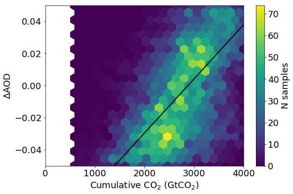
[19]:
from esem.sampler import MCMCSampler

# The MCMC algorithm works much better with a normalised parameter range, so recreate the model
m = gp_model(pd.concat([df[['co2']]/4000, (df[['od550aer']]+0.05)/0.1], axis=1), df[['tas']].values, kernel=['Linear'])
m.train()

# Target 1.2 degrees above present day (roughly 2 degrees above pre-industrial)
sampler = MCMCSampler(m, np.asarray([1.2], dtype=np.float64))
samples = sampler.sample(n_samples=8000, mcmc_kwargs=dict(num_burnin_steps=1000) )
Acceptance rate: 0.9614173964786951
[20]:
# Get the emulated temperatures for these samples
new_samples = pd.DataFrame(data=samples, columns=['co2', 'od550aer'])
Z, _ = m.predict(new_samples.values)
[21]:
fig = plt.figure(figsize=(9, 6))

cl = plt.contour(xx, yy, Y_new.reshape(xx.shape), levels = [1.2],
             colors=('k',),linestyles=('-',),linewidths=(2,))

cl=plt.hexbin(new_samples.co2*4000, new_samples.od550aer*0.1-0.05, gridsize=20)

plt.setp(plt.gca(), xlabel='Cumulative CO$_2$ (GtCO$_2$)', ylabel='$\Delta$AOD')

plt.colorbar(cl, label='N samples')
plt.setp(plt.gca(), ylim=[-0.05, 0.05], xlim=[0, 4000])

plt.savefig('CMIP6_emulator_sampled.png', transparent=True)
[ ]: