Calibrating GPs using ABC
[1]:
import warnings
warnings.filterwarnings('ignore') # Ignore all the iris warnings...
[2]:
import pandas as pd
import cis
import iris

from utils import get_aeronet_data, get_bc_ppe_data

from esem.utils import validation_plot, plot_parameter_space, get_random_params, ensemble_collocate
from esem import gp_model
from esem.abc_sampler import ABCSampler, constrain

import iris.quickplot as qplt
import matplotlib.pyplot as plt
%matplotlib inline
Read in the parameters and observables
[3]:
aaod = get_aeronet_data()
print(aaod)
Ungridded data: Absorption_AOD440nm / (1)
     Shape = (10098,)

     Total number of points = 10098
     Number of non-masked points = 10098
     Long name = Absorption_AOD440nm
     Standard name = None
     Units = 1
     Missing value = -999.0
     Range = (5.1e-05, 0.47236)
     History =
     Coordinates:
       longitude
          Long name =
          Standard name = longitude
          Units = degrees_east
          Missing value = None
          Range = (-155.576755, 141.3407)
          History =
       latitude
          Long name =
          Standard name = latitude
          Units = degrees_north
          Missing value = None
          Range = (-35.495807, 79.990278)
          History =
       time
          Long name =
          Standard name = time
          Units = days since 1600-01-01 00:00:00
          Missing value = None
          Range = (cftime.DatetimeGregorian(2017, 1, 1, 12, 0, 0, 0, has_year_zero=False), cftime.DatetimeGregorian(2018, 1, 2, 12, 0, 0, 0, has_year_zero=False))
          History =
[4]:
# Read in the PPE parameters, AAOD and DRE
ppe_params, ppe_aaod, ppe_dre = get_bc_ppe_data(dre=True)
[5]:
# Take the annual mean of the DRE
ppe_dre, = ppe_dre.collapsed('time', iris.analysis.MEAN)
WARNING:root:Creating guessed bounds as none exist in file
WARNING:root:Creating guessed bounds as none exist in file
WARNING:root:Creating guessed bounds as none exist in file
WARNING:root:Creating guessed bounds as none exist in file
Collocate the model on to the observations
[6]:
col_ppe_aaod = ensemble_collocate(ppe_aaod, aaod)
[7]:
n_test = 8

X_test, X_train = ppe_params[:n_test], ppe_params[n_test:]
Y_test, Y_train = col_ppe_aaod[:n_test], col_ppe_aaod[n_test:]
[8]:
Y_train
[8]:
| Absorption Optical Thickness - Total 550Nm (1) | job | obs |
|---|---|---|
| Shape | 31 | 10098 |
| Dimension coordinates | ||
| job | x | - |
| obs | - | x |
| Auxiliary coordinates | ||
| latitude | - | x |
| longitude | - | x |
| time | - | x |
Setup and run the models
Explore different model choices
[9]:
from esem.utils import leave_one_out, prediction_within_ci
from scipy import stats
import numpy as np

from esem.data_processors import Log
res_l = leave_one_out(X_train, Y_train, model='GaussianProcess', data_processors=[Log(constant=0.1)], kernel=['Linear', 'Exponential', 'Bias'])
r2_values_l = [stats.linregress(x.data.compressed(), y.data[:, ~x.data.mask].flatten())[2]**2 for x,y,_ in res_l]
ci95_values_l = [prediction_within_ci(x.data.flatten(), y.data.flatten(), v.data.flatten())[2].sum()/x.data.count() for x,y,v in res_l]
print("Mean R^2: {:.2f}".format(np.asarray(r2_values_l).mean()))
print("Mean proportion within 95% CI: {:.2f}".format(np.asarray(ci95_values_l).mean()))

res = leave_one_out(X_train, Y_train, model='GaussianProcess', kernel=['Linear', 'Bias'])
r2_values = [stats.linregress(x.data.flatten(), y.data.flatten())[2]**2 for x,y,v in res]
ci95_values = [prediction_within_ci(x.data.flatten(), y.data.flatten(), v.data.flatten())[2].sum()/x.data.count() for x,y,v in res]
print("Mean R^2: {:.2f}".format(np.asarray(r2_values).mean()))
print("Mean proportion within 95% CI: {:.2f}".format(np.asarray(ci95_values).mean()))

# Note that while the Log pre-processing leads to slightly better R^2, the model is under-confident and
#  has too large uncertainties which would adversley effec our implausibility metric.
Mean R^2: 1.00
Mean proportion within 95% CI: 1.00
Mean R^2: 0.99
Mean proportion within 95% CI: 0.94
Build final model
[10]:
model = gp_model(X_train, Y_train, kernel=['Linear', 'Bias'])
[11]:
model.train()
[12]:
m, v = model.predict(X_test.values)
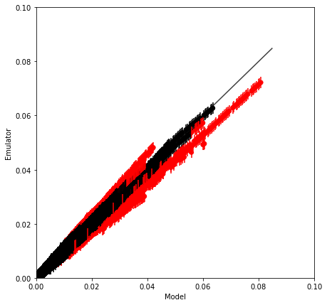
[13]:
validation_plot(Y_test.data.flatten(), m.data.flatten(), v.data.flatten(),
               minx=0, maxx=0.1, miny=0., maxy=0.1)
Proportion of 'Bad' estimates : 5.52%
Sample and constrain the models
Emulating 1e6 sample points directly would require 673 Gb of memory so we can either run 1e6 samples for each point, or run the constraint everywhere, but in batches. Here we do the latter, optioanlly on the GPU, using the ‘naive’ algorithm for calculating the running mean and variance of the various properties.
The rejection sampling happens in a similar manner so that only as much memory as is used for one batch is ever used.
[14]:
# In this case
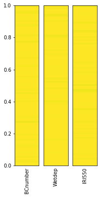
sample_points = pd.DataFrame(data=get_random_params(3, int(1e6)), columns=X_train.columns)
[15]:
# Note that smoothing the parameter distribution can be slow for large numbers of points
plot_parameter_space(sample_points, fig_size=(3,6), smooth=False)
[16]:
# Setup the sampler to compare against our AeroNet data
sampler = ABCSampler(model, aaod, obs_uncertainty=0.5, repres_uncertainty=0.5)
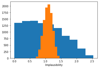
[17]:
# Calculate the implausibilty for each sample against each observation - note this can be very large so we only sample a fraction!
implaus = sampler.get_implausibility(sample_points[::100], batch_size=1000)

# The implausibility distributions for different observations can be very different.
_ = plt.hist(implaus.data[:, 1400])
_ = plt.hist(implaus.data[:, 14])
plt.gca().set(xlabel='Implausibility')
<tqdm.auto.tqdm object at 0x00000236A10BA5E0>
[17]:
[Text(0.5, 0, 'Implausibility')]
[18]:
# Find the valid samples in our full 1million samples by comparing against a given tolerance and threshold
valid_samples = sampler.batch_constrain(sample_points, batch_size=10000, tolerance=.1)
print("Remaining points: {}".format(valid_samples.sum()))
<tqdm.auto.tqdm object at 0x000002398006DC70>Remaining points: 729474
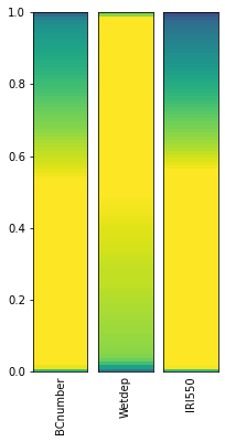
[19]:
# Plot the reduced parameter distribution
constrained_sample = sample_points[valid_samples]
plot_parameter_space(constrained_sample, fig_size=(3,6))
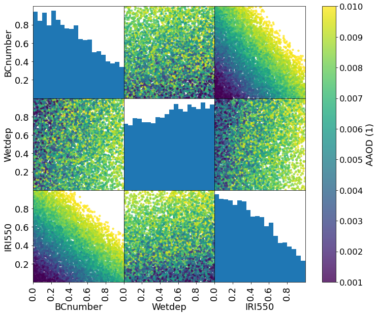
[20]:
# We can also easily plot the joint distributions
#  Only plot every one in 100 points as scatter plots with large numbers of points are slow...
import matplotlib

# Mimic Seaborn scaling without requiring the whole package
scale = 1.5
matplotlib.rcParams['font.size'] = 12 * scale
matplotlib.rcParams['axes.labelsize'] = 12 * scale
matplotlib.rcParams['axes.titlesize'] = 12 * scale
matplotlib.rcParams['xtick.labelsize'] = 11 * scale
matplotlib.rcParams['ytick.labelsize'] = 11 * scale
matplotlib.rcParams['lines.linewidth'] = 1.5 * scale
matplotlib.rcParams['lines.markersize'] = 6 * scale
#

m, _ = model.predict(constrained_sample[::100].values)
Zs = m.data
# Plot the emulated AAOD value (averaged over observation locations) for each point
grr = pd.plotting.scatter_matrix(constrained_sample[::100], c=Zs.mean(axis=1), figsize=(12, 10), marker='o',
                                 hist_kwds={'bins': 20,}, s=20, alpha=.8, vmin=1e-3, vmax=1e-2, range_padding=0.,
                                 density_kwds={'range': [[0., 1.], [0., 1.]], 'colormap':'viridis'},
                                 )

# Matplotlib dragons...
grr[0][0].set_yticklabels([0.2, 0.4, 0.6, 0.8], fontsize=12 * scale)
for i in range(2):
    grr[i+1][0].set_yticklabels([0.0, 0.2, 0.4, 0.6, 0.8], fontsize=12 * scale)
for i in range(3):
    grr[2][i].set_xticks([0.0, 0.2, 0.4, 0.6, 0.8])
    grr[2][i].set_xticklabels([0.0, 0.2, 0.4, 0.6, 0.8], fontsize=12 * scale)

plt.colorbar(grr[0][1].collections[0], ax=grr, use_gridspec=True, label='AAOD (1)')

plt.savefig('BCPPE_constrained_params_paper.png', transparent=True)
Explore the uncertainty in Direct Radiative Effect of Aerosol in constrianed sample-space
[21]:
dre_test, dre_train = ppe_dre[:n_test], ppe_dre[n_test:]

ari_model = gp_model(X_train, dre_train, name="ARI", kernel=['Linear', 'Bias'])
ari_model.train()
[22]:
# Calculate the mean and std-dev DRE over each set of sample points

unconstrained_mean_ari, unconstrained_sd_ari = ari_model.batch_stats(sample_points, batch_size=10000)
constrained_mean_ari, constrained_sd_ari = ari_model.batch_stats(constrained_sample, batch_size=10000)
<tqdm.auto.tqdm object at 0x00000239A2B2D310>
<tqdm.auto.tqdm object at 0x00000239ACFEFDF0>
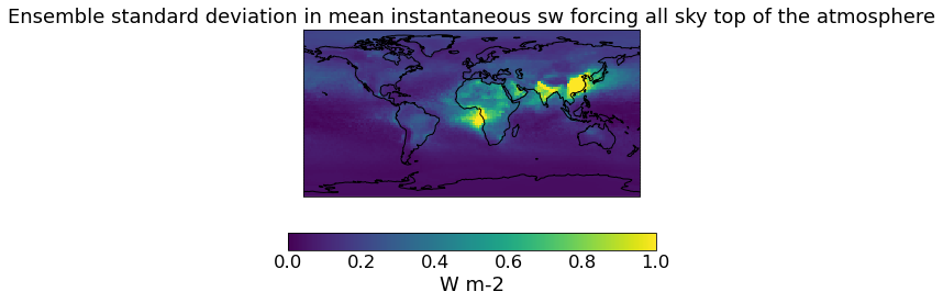
[23]:
# The original (unconstrained DRE)
qplt.pcolormesh(unconstrained_sd_ari, vmin=0., vmax=1)
plt.gca().coastlines()
[23]:
<cartopy.mpl.feature_artist.FeatureArtist at 0x239ad149610>
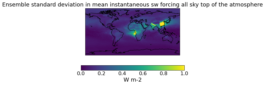
[24]:
# The constrained DRE
qplt.pcolormesh(constrained_sd_ari, vmin=0., vmax=1)
plt.gca().coastlines()
[24]:
<cartopy.mpl.feature_artist.FeatureArtist at 0x239af7e3700>
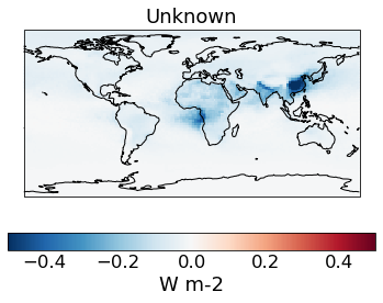
[25]:
# The change in spread after the constraint is applied
qplt.pcolormesh((constrained_sd_ari-unconstrained_sd_ari), cmap='RdBu_r', vmin=-5e-1, vmax=5e-1)
plt.gca().coastlines()
[25]:
<cartopy.mpl.feature_artist.FeatureArtist at 0x239af86c310>
[ ]: